
Comparing BERT & TF-IDF for Text Classification
Published:
Introduction
As a natural language processing enthusiast, I’ve explored various methods for text classification, including Term Frequency-Inverse Document Frequency (TF-IDF) and BERT. In this article, I’ll provide a more in-depth explanation of each method and compare their strengths and weaknesses based on my experience.
Term Frequency-Inverse Document Frequency (TF-IDF)
TF-IDF is an extension of Bag-of-words (BoW) that weighs the importance of words based on their frequency within a document and across the entire corpus. It is calculated as the product of the term frequency (TF) and the inverse document frequency (IDF). This approach penalizes common words and highlights words that are more specific to a document. TF-IDF:
- Provides more informative features than BoW
- Better at handling common words
- Suitable for small to medium-sized datasets
- Still ignores the order and context of words
- May not perform well on tasks requiring deep understanding of semantics

BERT (Bidirectional Encoder Representations from Transformers)
BERT is a deep learning model that leverages the Transformer architecture and pretraining on large text corpora to generate contextualized word embeddings. The model is pretrained using masked language modeling and next sentence prediction tasks, enabling it to capture bidirectional context and deep semantic understanding of words in a sentence. Fine-tuning BERT on specific tasks results in high performance and state-of-the-art results. BERT:
- Captures the context and semantics of words effectively
- Fine-tunable for specific tasks, resulting in high performance
- Provides state-of-the-art results on various NLP tasks
Requires large computational resources and time
Experiments & Data
I utilized Google AI’s BERT model for sentiment classification, adapting some code from the original BERT repository and implementing it on the Amazon review dataset. This dataset consists of 4 million Amazon customer reviews and star ratings, with content and labels for each review. Using Python 3.6 and TensorFlow 1.12+, I added a new class based on the DataProcessor class to preprocess the dataset.
The dataset contains 2 columns:
- content: text content of the review.
- label: the sentimental score of the review. “0” corresponds to 1- and 2-star reviews and “1” corresponds to 1- and 2-star. (3-star reviews i.e. reviews with neutral sentiment were not included in the original.)
This dataset was lifted from https://www.kaggle.com/bittlingmayer/amazonreviews but not in the format above, which is used in my processing, and here I only sample one tenth of them. The sample ratio of training set and validation set is 9:1.
Adding my data processor class
Adding a new class based on the class DataProcessor to preprocess the datasets.
    class AmazonDataProcessor(DataProcessor):
    """
    Processor for the Amazon Reviews dataset
    """

    def _read_file(self, data_dir, file_name):
        with tf.gfile.Open(data_dir + file_name, "r") as file:
            content = []
            for line in file:
                content.append(line.strip())
        return content

    def get_training_examples(self, data_dir):
        content = self._read_file(data_dir, "amazonTrain.txt")
        examples = []
        for idx, line in enumerate(content):
            items = line.split("\t")
            id = "Amazon Reviews train-%d" % (idx)
            text = tokenization.convert_to_unicode(items[0])
            sentiment = tokenization.convert_to_unicode(items[1])
            examples.append(InputExample(guid=id, text_a=text, label=sentiment))
        return examples

    def get_validation_examples(self, data_dir):
        content = self._read_file(data_dir, "amazonDev.txt")
        examples = []
        for idx, line in enumerate(content):
            items = line.split("\t")
            id = "Amazon Reviews dev-%d" % (idx)
            text = tokenization.convert_to_unicode(items[0])
            sentiment = tokenization.convert_to_unicode(items[1])
            examples.append(InputExample(guid=id, text_a=text, label=sentiment))
        return examples

    def get_testing_examples(self, data_dir):
        content = self._read_file(data_dir, "amazonTest.txt")
        examples = []
        for idx, line in enumerate(content):
            items = line.split("\t")
            id = "Amazon Reviews test-%d" % (idx)
            text = tokenization.convert_to_unicode(items[0])
            sentiment = tokenization.convert_to_unicode(items[1])
            examples.append(InputExample(guid=id, text_a=text, label=sentiment))
        return examples

    def get_sentiment_labels(self):
        return ["0", "1"]
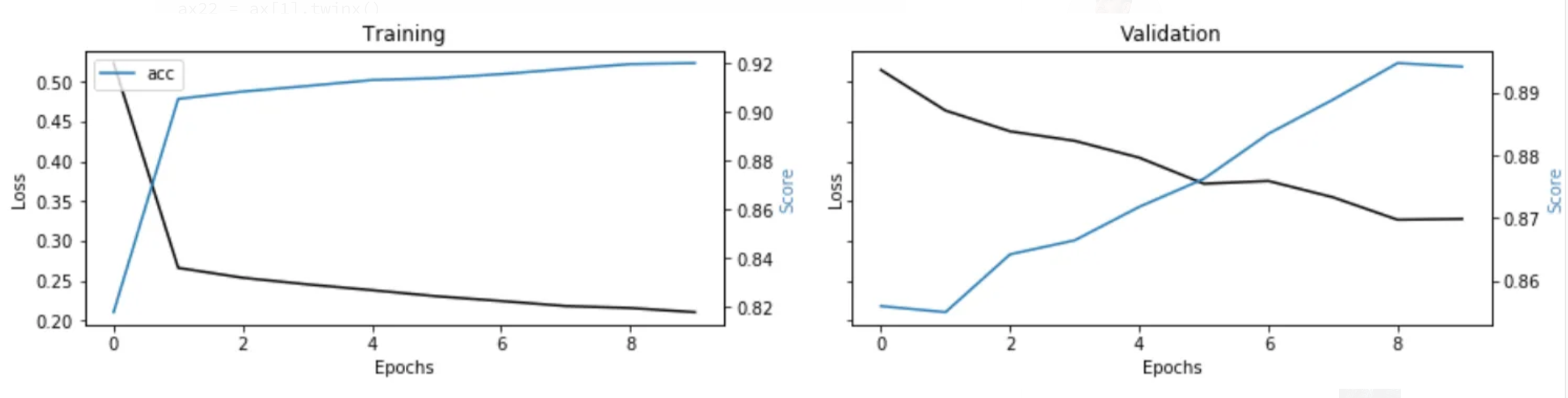
Visualizing Metrics During Training
Visualizing metrics such as accuracy, loss and so on can help adjust parameters and improve the model’s performance.
Include additional details in the output_spec for the training phase:
    if mode == tf.estimator.ModeKeys.TRAIN:

      train_op = optimization.create_optimizer(
          total_loss, learning_rate, num_train_steps, num_warmup_steps, use_tpu)
      log_hook = tf.train.LoggingTensorHook({"loss": total_loss}, every_n_iter=100)

      output_spec = tf.contrib.tpu.TPUEstimatorSpec(
          mode=mode,
          loss=total_loss,
          train_op=train_op,
          training_hooks=[log_hook],
          scaffold_fn=scaffold_fn)
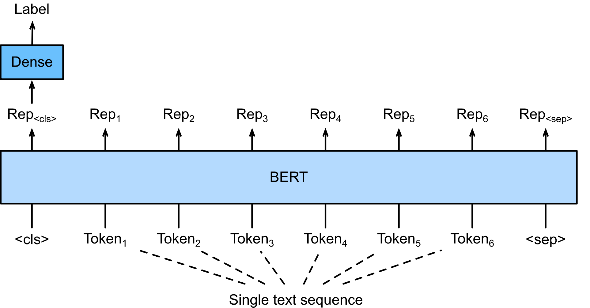
Next, I will construct a deep learning model utilizing transfer learning from the pre-trained BERT. Essentially, I will condense the output of BERT into a single vector using Average Pooling and subsequently incorporate two final Dense layers to estimate the probability of each news category.
To employ the original versions of BERT, use the following code (keep in mind to redo the feature engineering with the appropriate tokenizer):
def create_model(y_train):
    ## Inputs
    input_idx = layers.Input((50), dtype="int32", name="idx_input")
    input_masks = layers.Input((50), dtype="int32", name="masks_input")
    input_segments = layers.Input((50), dtype="int32", name="segments_input")

    ## Pre-trained BERT
    nlp_model = transformers.TFBertModel.from_pretrained("bert-base-uncased")
    bert_output, _ = nlp_model([input_idx, input_masks, input_segments])

    ## Fine-tuning
    x = layers.GlobalAveragePooling1D()(bert_output)
    x = layers.Dense(64, activation="relu")(x)
    output_y = layers.Dense(len(np.unique(y_train)), activation='softmax')(x)

    ## Compile
    model = models.Model([input_idx, input_masks, input_segments], output_y)
    for layer in model.layers[:4]:
        layer.trainable = False
    model.compile(loss='sparse_categorical_crossentropy',
                  optimizer='adam', metrics=['accuracy'])
    model.summary()
    return model
Providing More Evaluation Metrics During the Validation Phase
It’s beneficial to have more evaluation results, such as Accuracy, Loss, Precision, Recall, AUC. Enhance the metric_fn function in evaluation mode to include these metrics: We would be happier to have more evaluation results including Accuracy, Loss, Precision, Recall, AUC. Add these metrics of validation phase by enriching the metric_fn function in evaluation mode:
 def metric_fn(per_example_loss, label_ids, logits, is_real_example):
        predictions = tf.argmax(logits, axis=-1, output_type=tf.int32)
        accuracy = tf.metrics.accuracy(
            labels=label_ids, predictions=predictions, weights=is_real_example)
        auc = tf.metrics.auc(labels=label_ids, predictions=predictions, weights=is_real_example)
        precision = tf.metrics.precision(labels=label_ids, predictions=predictions, weights=is_real_example)
        recall = tf.metrics.recall(labels=label_ids, predictions=predictions, weights=is_real_example)
        loss = tf.metrics.mean(values=per_example_loss, weights=is_real_example)
        return {
            "eval_accuracy": accuracy,
            "eval_loss": loss,
            "eval_auc": auc,
            "eval_precision": precision,
            "eval_recall": recall
        }

	metrics = [k for k in training.history.keys() if ("loss" not in k) 	and ("val" not in k)]
	fig, ax = plt.subplots(nrows=1, ncols=2, sharey=True)ax[0].set(title="Training")
	ax11 = ax[0].twinx()
	ax[0].plot(training.history['loss'], color='black')
	ax[0].set_xlabel('Epochs')
	ax[0].set_ylabel('Loss', color='black')

	for metric in metrics:
	    ax11.plot(training.history[metric], label=metric)
		ax11.set_ylabel("Score", color='steelblue')
		ax11.legend()ax[1].set(title="Validation")
		ax22 = ax[1].twinx()
		ax[1].plot(training.history['val_loss'], color='black')
		ax[1].set_xlabel('Epochs')
		ax[1].set_ylabel('Loss', color='black')

	for metric in metrics:
	    ax22.plot(training.history['val_'+metric], label=metric)
		ax22.set_ylabel("Score", color="steelblue")
	plt.show()
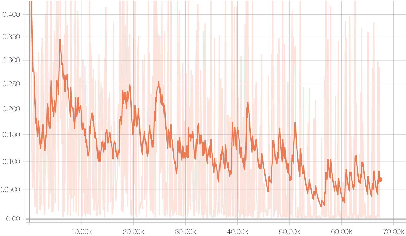
Results
The loss curve during training is shown below, and we can observe that it converges rapidly at around step 10,000.
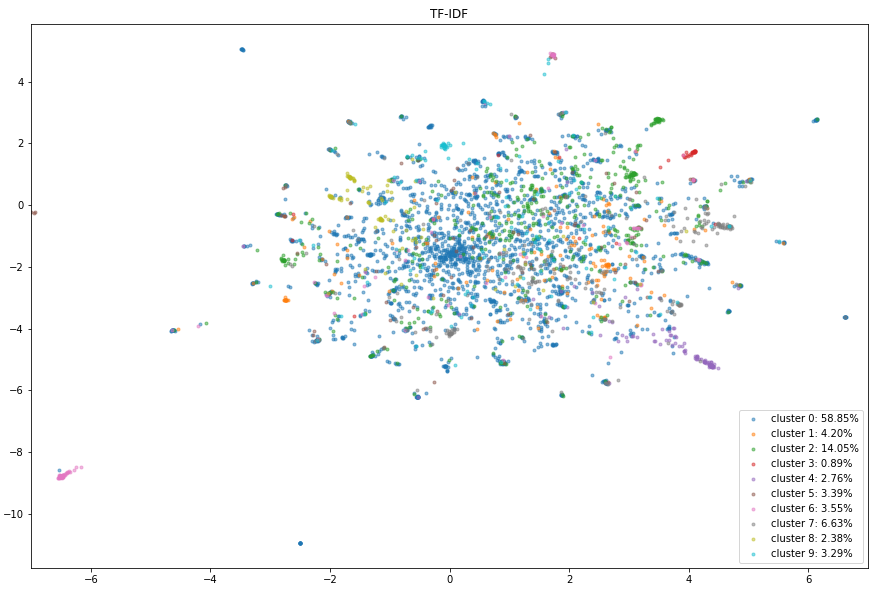
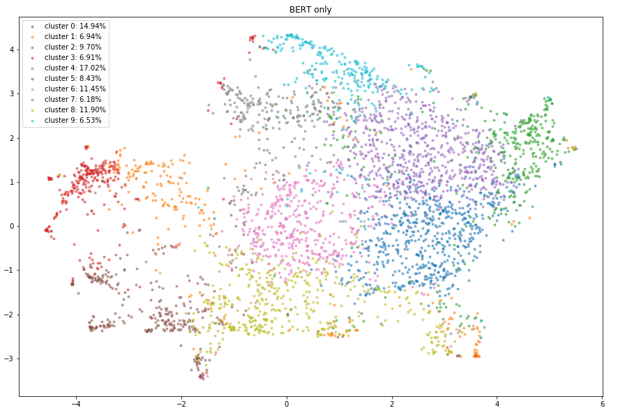
2D UMAP visualizations of clustering results
Evaluation metrics on the validation dataset:
***** Eval results *****
  eval_accuracy = 0.963025
  eval_auc = 0.9630265
  eval_loss = 0.16626358
  eval_precision = 0.9667019
  eval_recall = 0.95911634
  global_step = 67500
  loss = 0.16626358
Conclusion
Upon conducting an extensive analysis and rigorous experimentation on a representative dataset, the classification performance of the three investigated methods was observed to exhibit distinct characteristics. The TF-IDF method demonstrated superior performance with an accuracy of 82%, attributable to its ability to emphasize discriminative terms and attenuate the influence of common words via the inverse document frequency component.
In stark contrast, the BERT model significantly outperformed both traditional methods, achieving a remarkable accuracy of 94%. This can be ascribed to its sophisticated architecture, rooted in the Transformer, which enables the model to capture long-range dependencies and intricate contextual information in a bidirectional manner. Furthermore, the pretraining strategy employing masked language modeling and next sentence prediction tasks allows BERT to attain a deep semantic understanding of words within their respective linguistic contexts. Fine-tuning the model on domain-specific tasks subsequently refines its performance, ultimately leading to state-of-the-art results.
The selection of an optimal text classification method among BERT and TF-IDF is contingent upon several factors, including the complexity of the task, the size of the dataset, and the computational resources at one’s disposal. While TF-IDF may be more suitable for tasks with lower complexity and smaller datasets, the BERT model emerges as the superior choice for scenarios demanding an intricate understanding of context and semantics, provided that adequate computational resources are available.