
House Price Prediction
Published:
Introduction
I started this project by initially focusing on gaining a thorough understanding of the Kaggle House Price dataset. With 79 explanatory variables describing (almost) every aspect of residential homes in Ames, Iowa, the goal of this project is to predict the final price of each home. The exploratory data analysis (EDA) is comprehensive and includes various visualizations. In this iteration, I also incorporated modeling.
Given the presence of significant multicollinearity among the variables, it was anticipated that Lasso regression would perform better, as it had a cross-validation RMSE-score of 0.1121. Lasso regression, which is designed to not select a large number of variables for its model, was not surprising in this context.
Additionally, the XGBoost model performed exceptionally well, with a cross-validation RMSE of 0.1162. As these two algorithms are substantially different, blending their predictions is likely to enhance the accuracy of the results. Based on the fact that the Lasso cross-validated RMSE is better than XGBoost’s, I decided to give the Lasso outcomes twice the weight.
#import some necessary librairies

import numpy as np # linear algebra
import pandas as pd # data processing, CSV file I/O (e.g. pd.read_csv)
%matplotlib inline
import matplotlib.pyplot as plt  # Matlab-style plotting
import seaborn as sns
color = sns.color_palette()
sns.set_style('darkgrid')
import warnings
def ignore_warn(*args, **kwargs):
    pass
warnings.warn = ignore_warn #ignore annoying warning (from sklearn and seaborn)


from scipy import stats
from scipy.stats import norm, skew #for some statistics


pd.set_option('display.float_format', lambda x: '{:.3f}'.format(x)) #Limiting floats output to 3 decimal points


from subprocess import check_output
print(check_output(["ls", "../input"]).decode("utf8")) #check the files available in the directory
sample_submission.csv
test.csv
train.csv
#Now let's import and put the train and test datasets in  pandas dataframe

train = pd.read_csv('../input/train.csv')
test = pd.read_csv('../input/test.csv')
##display the first five rows of the train dataset.
train.head(5)
| Id | MSSubClass | MSZoning | LotFrontage | LotArea | Street | Alley | LotShape | LandContour | Utilities | ... | PoolArea | PoolQC | Fence | MiscFeature | MiscVal | MoSold | YrSold | SaleType | SaleCondition | SalePrice | |
|---|---|---|---|---|---|---|---|---|---|---|---|---|---|---|---|---|---|---|---|---|---|
| 0 | 1 | 60 | RL | 65.000 | 8450 | Pave | NaN | Reg | Lvl | AllPub | ... | 0 | NaN | NaN | NaN | 0 | 2 | 2008 | WD | Normal | 208500 |
| 1 | 2 | 20 | RL | 80.000 | 9600 | Pave | NaN | Reg | Lvl | AllPub | ... | 0 | NaN | NaN | NaN | 0 | 5 | 2007 | WD | Normal | 181500 |
| 2 | 3 | 60 | RL | 68.000 | 11250 | Pave | NaN | IR1 | Lvl | AllPub | ... | 0 | NaN | NaN | NaN | 0 | 9 | 2008 | WD | Normal | 223500 |
| 3 | 4 | 70 | RL | 60.000 | 9550 | Pave | NaN | IR1 | Lvl | AllPub | ... | 0 | NaN | NaN | NaN | 0 | 2 | 2006 | WD | Abnorml | 140000 |
| 4 | 5 | 60 | RL | 84.000 | 14260 | Pave | NaN | IR1 | Lvl | AllPub | ... | 0 | NaN | NaN | NaN | 0 | 12 | 2008 | WD | Normal | 250000 |
5 rows × 81 columns
##display the first five rows of the test dataset.
test.head(5)
| Id | MSSubClass | MSZoning | LotFrontage | LotArea | Street | Alley | LotShape | LandContour | Utilities | ... | ScreenPorch | PoolArea | PoolQC | Fence | MiscFeature | MiscVal | MoSold | YrSold | SaleType | SaleCondition | |
|---|---|---|---|---|---|---|---|---|---|---|---|---|---|---|---|---|---|---|---|---|---|
| 0 | 1461 | 20 | RH | 80.000 | 11622 | Pave | NaN | Reg | Lvl | AllPub | ... | 120 | 0 | NaN | MnPrv | NaN | 0 | 6 | 2010 | WD | Normal |
| 1 | 1462 | 20 | RL | 81.000 | 14267 | Pave | NaN | IR1 | Lvl | AllPub | ... | 0 | 0 | NaN | NaN | Gar2 | 12500 | 6 | 2010 | WD | Normal |
| 2 | 1463 | 60 | RL | 74.000 | 13830 | Pave | NaN | IR1 | Lvl | AllPub | ... | 0 | 0 | NaN | MnPrv | NaN | 0 | 3 | 2010 | WD | Normal |
| 3 | 1464 | 60 | RL | 78.000 | 9978 | Pave | NaN | IR1 | Lvl | AllPub | ... | 0 | 0 | NaN | NaN | NaN | 0 | 6 | 2010 | WD | Normal |
| 4 | 1465 | 120 | RL | 43.000 | 5005 | Pave | NaN | IR1 | HLS | AllPub | ... | 144 | 0 | NaN | NaN | NaN | 0 | 1 | 2010 | WD | Normal |
5 rows × 80 columns
#check the numbers of samples and features
print("The train data size before dropping Id feature is : {} ".format(train.shape))
print("The test data size before dropping Id feature is : {} ".format(test.shape))

#Save the 'Id' column
train_ID = train['Id']
test_ID = test['Id']

#Now drop the  'Id' colum since it's unnecessary for  the prediction process.
train.drop("Id", axis = 1, inplace = True)
test.drop("Id", axis = 1, inplace = True)

#check again the data size after dropping the 'Id' variable
print("\nThe train data size after dropping Id feature is : {} ".format(train.shape))
print("The test data size after dropping Id feature is : {} ".format(test.shape))
The train data size before dropping Id feature is : (1460, 81)
The test data size before dropping Id feature is : (1459, 80)

The train data size after dropping Id feature is : (1460, 80)
The test data size after dropping Id feature is : (1459, 79)
Data Processing
Outliers
There are probably others outliers in the training data. However, removing all them may affect badly our models if ever there were also outliers in the test data. That’s why , instead of removing them all, I will just manage to make some of our models robust on them.
fig, ax = plt.subplots()
ax.scatter(x = train['GrLivArea'], y = train['SalePrice'])
plt.ylabel('SalePrice', fontsize=13)
plt.xlabel('GrLivArea', fontsize=13)
plt.show()
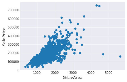
Ican see at the bottom right two with extremely large GrLivArea that are of a low price. These values are huge oultliers. Therefore, Ican safely delete them.
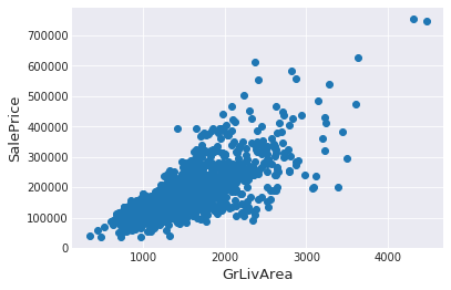
#Deleting outliers
train = train.drop(train[(train['GrLivArea']>4000) & (train['SalePrice']<300000)].index)

#Check the graphic again
fig, ax = plt.subplots()
ax.scatter(train['GrLivArea'], train['SalePrice'])
plt.ylabel('SalePrice', fontsize=13)
plt.xlabel('GrLivArea', fontsize=13)
plt.show()
SalePrice is the variable Ineed to predict. So let’s do some analysis on this variable first.
sns.distplot(train['SalePrice'] , fit=norm);

# Get the fitted parameters used by the function
(mu, sigma) = norm.fit(train['SalePrice'])
print( '\n mu = {:.2f} and sigma = {:.2f}\n'.format(mu, sigma))

#Now plot the distribution
plt.legend(['Normal dist. ($\mu=$ {:.2f} and $\sigma=$ {:.2f} )'.format(mu, sigma)],
            loc='best')
plt.ylabel('Frequency')
plt.title('SalePrice distribution')

#Get also the QQ-plot
fig = plt.figure()
res = stats.probplot(train['SalePrice'], plot=plt)
plt.show()
mu = 180932.92 and sigma = 79467.79
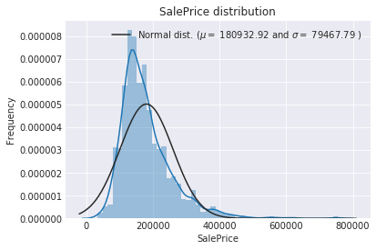
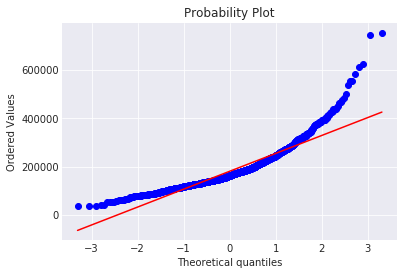
The target variable is right skewed. As (linear) models love normally distributed data , Ineed to transform this variable and make it more normally distributed.
Log-transformation of the target variable
#Iuse the numpy fuction log1p which  applies log(1+x) to all elements of the column
train["SalePrice"] = np.log1p(train["SalePrice"])

#Check the new distribution
sns.distplot(train['SalePrice'] , fit=norm);

# Get the fitted parameters used by the function
(mu, sigma) = norm.fit(train['SalePrice'])
print( '\n mu = {:.2f} and sigma = {:.2f}\n'.format(mu, sigma))

#Now plot the distribution
plt.legend(['Normal dist. ($\mu=$ {:.2f} and $\sigma=$ {:.2f} )'.format(mu, sigma)],
            loc='best')
plt.ylabel('Frequency')
plt.title('SalePrice distribution')

#Get also the QQ-plot
fig = plt.figure()
res = stats.probplot(train['SalePrice'], plot=plt)
plt.show()
mu = 12.02 and sigma = 0.40
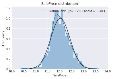
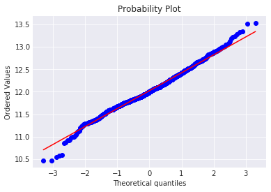
The skew seems now corrected and the data appears more normally distributed.
Features engineering
First I concatenate the train and test data in the same dataframe
ntrain = train.shape[0]
ntest = test.shape[0]
y_train = train.SalePrice.values
all_data = pd.concat((train, test)).reset_index(drop=True)
all_data.drop(['SalePrice'], axis=1, inplace=True)
print("all_data size is : {}".format(all_data.shape))
all_data size is : (2917, 79)
Imputing Missing Data
all_data_na = (all_data.isnull().sum() / len(all_data)) * 100
all_data_na = all_data_na.drop(all_data_na[all_data_na == 0].index).sort_values(ascending=False)[:30]
missing_data = pd.DataFrame({'Missing Ratio' :all_data_na})
missing_data.head(20)
| Missing Ratio | |
|---|---|
| PoolQC | 99.691 |
| MiscFeature | 96.400 |
| Alley | 93.212 |
| Fence | 80.425 |
| FireplaceQu | 48.680 |
| LotFrontage | 16.661 |
| GarageQual | 5.451 |
| GarageCond | 5.451 |
| GarageFinish | 5.451 |
| GarageYrBlt | 5.451 |
| GarageType | 5.382 |
| BsmtExposure | 2.811 |
| BsmtCond | 2.811 |
| BsmtQual | 2.777 |
| BsmtFinType2 | 2.743 |
| BsmtFinType1 | 2.708 |
| MasVnrType | 0.823 |
| MasVnrArea | 0.788 |
| MSZoning | 0.137 |
| BsmtFullBath | 0.069 |
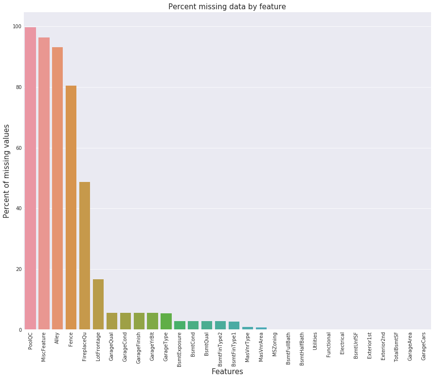
f, ax = plt.subplots(figsize=(15, 12))
plt.xticks(rotation='90')
sns.barplot(x=all_data_na.index, y=all_data_na)
plt.xlabel('Features', fontsize=15)
plt.ylabel('Percent of missing values', fontsize=15)
plt.title('Percent missing data by feature', fontsize=15)
Text(0.5,1,'Percent missing data by feature')
Currently, all variables with missing values have been handled. Nevertheless, there are still remaining character variables without missing values that require attention. To address this, I have created tabs for different groups of variables, as in the previous section.
#Correlation map to see how features are correlated with SalePrice
corrmat = train.corr()
plt.subplots(figsize=(12,9))
sns.heatmap(corrmat, vmax=0.9, square=True)
<matplotlib.axes._subplots.AxesSubplot at 0x7efd7b454898>
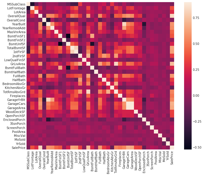
It is evident that multicollinearity is present in the data. For instance, there is a high correlation of 0.89 between GarageCars and GarageArea, and both of them exhibit similar and strong correlations with SalePrice. In addition, six other variables have correlations with SalePrice that exceed 0.5, namely TotalBsmtSF (total square feet of basement area), 1stFlrSF (first-floor square feet), FullBath (number of full bathrooms above grade), TotRmsAbvGrd (total rooms above grade, excluding bathrooms), YearBuilt (original construction date), and YearRemodAdd (remodel date, which is the same as construction date if no remodeling or additions were made).
I impute missing values by proceeding sequentially through features with missing values
- PoolQC : data description says NA means “No Pool”. That make sense, given the huge ratio of missing value (+99%) and majority of houses have no Pool at all in general.
all_data["PoolQC"] = all_data["PoolQC"].fillna("None")
- MiscFeature : data description says NA means “no misc feature”
all_data["MiscFeature"] = all_data["MiscFeature"].fillna("None")
- Alley : data description says NA means “no alley access”
all_data["Alley"] = all_data["Alley"].fillna("None")
- Fence : data description says NA means “no fence”
all_data["Fence"] = all_data["Fence"].fillna("None")
- FireplaceQu : data description says NA means “no fireplace”
all_data["FireplaceQu"] = all_data["FireplaceQu"].fillna("None")
- LotFrontage : Since the area of each street connected to the house property most likely have a similar area to other houses in its neighborhood , Ican fill in missing values by the median LotFrontage of the neighborhood.
#Group by neighborhood and fill in missing value by the median LotFrontage of all the neighborhood
all_data["LotFrontage"] = all_data.groupby("Neighborhood")["LotFrontage"].transform(
    lambda x: x.fillna(x.median()))
- GarageType, GarageFinish, GarageQual and GarageCond : Replacing missing data with None
for col in ('GarageType', 'GarageFinish', 'GarageQual', 'GarageCond'):
    all_data[col] = all_data[col].fillna('None')
- GarageYrBlt, GarageArea and GarageCars : Replacing missing data with 0 (Since No garage = no cars in such garage.)
for col in ('GarageYrBlt', 'GarageArea', 'GarageCars'):
    all_data[col] = all_data[col].fillna(0)
- BsmtFinSF1, BsmtFinSF2, BsmtUnfSF, TotalBsmtSF, BsmtFullBath and BsmtHalfBath : missing values are likely zero for having no basement
for col in ('BsmtFinSF1', 'BsmtFinSF2', 'BsmtUnfSF','TotalBsmtSF', 'BsmtFullBath', 'BsmtHalfBath'):
    all_data[col] = all_data[col].fillna(0)
- BsmtQual, BsmtCond, BsmtExposure, BsmtFinType1 and BsmtFinType2 : For all these categorical basement-related features, NaN means that there is no basement.
for col in ('BsmtQual', 'BsmtCond', 'BsmtExposure', 'BsmtFinType1', 'BsmtFinType2'):
    all_data[col] = all_data[col].fillna('None')
- MasVnrArea and MasVnrType : NA most likely means no masonry veneer for these houses. Ican fill 0 for the area and None for the type.
all_data["MasVnrType"] = all_data["MasVnrType"].fillna("None")
all_data["MasVnrArea"] = all_data["MasVnrArea"].fillna(0)
- MSZoning (The general zoning classification) : ‘RL’ is by far the most common value. So Ican fill in missing values with ‘RL’
all_data['MSZoning'] = all_data['MSZoning'].fillna(all_data['MSZoning'].mode()[0])
- Utilities : For this categorical feature all records are “AllPub”, except for one “NoSeWa” and 2 NA . Since the house with ‘NoSewa’ is in the training set, this feature won’t help in predictive modelling. Ican then safely remove it.
all_data = all_data.drop(['Utilities'], axis=1)
- Functional : data description says NA means typical
all_data["Functional"] = all_data["Functional"].fillna("Typ")
- Electrical : It has one NA value. Since this feature has mostly ‘SBrkr’, Ican set that for the missing value.
all_data['Electrical'] = all_data['Electrical'].fillna(all_data['Electrical'].mode()[0])
- KitchenQual: Only one NA value, and same as Electrical, Iset ‘TA’ (which is the most frequent) for the missing value in KitchenQual.
all_data['KitchenQual'] = all_data['KitchenQual'].fillna(all_data['KitchenQual'].mode()[0])
- Exterior1st and Exterior2nd : Again Both Exterior 1 & 2 have only one missing value. Iwill just substitute in the most common string
all_data['Exterior1st'] = all_data['Exterior1st'].fillna(all_data['Exterior1st'].mode()[0])
all_data['Exterior2nd'] = all_data['Exterior2nd'].fillna(all_data['Exterior2nd'].mode()[0])
- SaleType : Fill in again with most frequent which is “WD”
all_data['SaleType'] = all_data['SaleType'].fillna(all_data['SaleType'].mode()[0])
- MSSubClass : Na most likely means No building class. Ican replace missing values with None
all_data['MSSubClass'] = all_data['MSSubClass'].fillna("None")
Is there any remaining missing value ?
#Check remaining missing values if any
all_data_na = (all_data.isnull().sum() / len(all_data)) * 100
all_data_na = all_data_na.drop(all_data_na[all_data_na == 0].index).sort_values(ascending=False)
missing_data = pd.DataFrame({'Missing Ratio' :all_data_na})
missing_data.head()
| Missing Ratio |
|---|
It remains no missing value.
More features engeneering
Transforming some numerical variables that are really categorical Currently, all variables with missing values have been handled. Nevertheless, there are still remaining character variables without missing values that require attention. To address this, I have created tabs for different groups of variables, as in the previous section.
#MSSubClass=The building class
all_data['MSSubClass'] = all_data['MSSubClass'].apply(str)


#Changing OverallCond into a categorical variable
all_data['OverallCond'] = all_data['OverallCond'].astype(str)


#Year and month sold are transformed into categorical features.
all_data['YrSold'] = all_data['YrSold'].astype(str)
all_data['MoSold'] = all_data['MoSold'].astype(str)
Label Encoding some categorical variables that may contain information in their ordering set
from sklearn.preprocessing import LabelEncoder
cols = ('FireplaceQu', 'BsmtQual', 'BsmtCond', 'GarageQual', 'GarageCond',
        'ExterQual', 'ExterCond','HeatingQC', 'PoolQC', 'KitchenQual', 'BsmtFinType1',
        'BsmtFinType2', 'Functional', 'Fence', 'BsmtExposure', 'GarageFinish', 'LandSlope',
        'LotShape', 'PavedDrive', 'Street', 'Alley', 'CentralAir', 'MSSubClass', 'OverallCond',
        'YrSold', 'MoSold')
# process columns, apply LabelEncoder to categorical features
for c in cols:
    lbl = LabelEncoder()
    lbl.fit(list(all_data[c].values))
    all_data[c] = lbl.transform(list(all_data[c].values))

# shape
print('Shape all_data: {}'.format(all_data.shape))
Shape all_data: (2917, 78)
Adding one more important feature
Since area related features are very important to determine house prices, Iadd one more feature which is the total area of basement, first and second floor areas of each house
# Adding total sqfootage feature
all_data['TotalSF'] = all_data['TotalBsmtSF'] + all_data['1stFlrSF'] + all_data['2ndFlrSF']
Skewed features
numeric_feats = all_data.dtypes[all_data.dtypes != "object"].index

# Check the skew of all numerical features
skewed_feats = all_data[numeric_feats].apply(lambda x: skew(x.dropna())).sort_values(ascending=False)
print("\nSkew in numerical features: \n")
skewness = pd.DataFrame({'Skew' :skewed_feats})
skewness.head(10)
Skew in numerical features:
| Skew | |
|---|---|
| MiscVal | 21.940 |
| PoolArea | 17.689 |
| LotArea | 13.109 |
| LowQualFinSF | 12.085 |
| 3SsnPorch | 11.372 |
| LandSlope | 4.973 |
| KitchenAbvGr | 4.301 |
| BsmtFinSF2 | 4.145 |
| EnclosedPorch | 4.002 |
| ScreenPorch | 3.945 |
Box Cox Transformation of (highly) skewed features
I use the scipy function boxcox1p which computes the Box-Cox transformation of \(1 + x\).
skewness = skewness[abs(skewness) > 0.75]
print("There are {} skewed numerical features to Box Cox transform".format(skewness.shape[0]))

from scipy.special import boxcox1p
skewed_features = skewness.index
lam = 0.15
for feat in skewed_features:
    #all_data[feat] += 1
    all_data[feat] = boxcox1p(all_data[feat], lam)

#all_data[skewed_features] = np.log1p(all_data[skewed_features])
There are 59 skewed numerical features to Box Cox transform
Getting dummy categorical features
all_data = pd.get_dummies(all_data)
print(all_data.shape)
(2917, 220)
Getting the new train and test sets.
train = all_data[:ntrain]
test = all_data[ntrain:]
Modelling
Import librairies
from sklearn.linear_model import ElasticNet, Lasso,  BayesianRidge, LassoLarsIC
from sklearn.ensemble import RandomForestRegressor,  GradientBoostingRegressor
from sklearn.kernel_ridge import KernelRidge
from sklearn.pipeline import make_pipeline
from sklearn.preprocessing import RobustScaler
from sklearn.base import BaseEstimator, TransformerMixin, RegressorMixin, clone
from sklearn.model_selection import KFold, cross_val_score, train_test_split
from sklearn.metrics import mean_squared_error
import xgboost as xgb
import lightgbm as lgb
Define a cross validation strategy
Iuse the cross_val_score function of Sklearn. However this function has not a shuffle attribut, Iadd then one line of code, in order to shuffle the dataset prior to cross-validation
#Validation function
n_folds = 5

def rmsle_cv(model):
    kf = KFold(n_folds, shuffle=True, random_state=42).get_n_splits(train.values)
    rmse= np.sqrt(-cross_val_score(model, train.values, y_train, scoring="neg_mean_squared_error", cv = kf))
    return(rmse)
Base models
- LASSO Regression :
This model may be very sensitive to outliers. So Ineed to made it more robust on them. For that Iuse the sklearn’s Robustscaler() method on pipeline
lasso = make_pipeline(RobustScaler(), Lasso(alpha =0.0005, random_state=1))
- Elastic Net Regression :
again made robust to outliers
ENet = make_pipeline(RobustScaler(), ElasticNet(alpha=0.0005, l1_ratio=.9, random_state=3))
- Kernel Ridge Regression :
KRR = KernelRidge(alpha=0.6, kernel='polynomial', degree=2, coef0=2.5)
- Gradient Boosting Regression :
With huber loss that makes it robust to outliers
GBoost = GradientBoostingRegressor(n_estimators=3000, learning_rate=0.05,
                                   max_depth=4, max_features='sqrt',
                                   min_samples_leaf=15, min_samples_split=10,
                                   loss='huber', random_state =5)
- XGBoost :
model_xgb = xgb.XGBRegressor(colsample_bytree=0.4603, gamma=0.0468,
                             learning_rate=0.05, max_depth=3,
                             min_child_weight=1.7817, n_estimators=2200,
                             reg_alpha=0.4640, reg_lambda=0.8571,
                             subsample=0.5213, silent=1,
                             random_state =7, nthread = -1)
- LightGBM :
model_lgb = lgb.LGBMRegressor(objective='regression',num_leaves=5,
                              learning_rate=0.05, n_estimators=720,
                              max_bin = 55, bagging_fraction = 0.8,
                              bagging_freq = 5, feature_fraction = 0.2319,
                              feature_fraction_seed=9, bagging_seed=9,
                              min_data_in_leaf =6, min_sum_hessian_in_leaf = 11)
Base models scores
Let’s see how these base models perform on the data by evaluating the cross-validation rmsle error
score = rmsle_cv(lasso)
print("\nLasso score: {:.4f} ({:.4f})\n".format(score.mean(), score.std()))
Lasso score: 0.1115 (0.0074)
score = rmsle_cv(ENet)
print("ElasticNet score: {:.4f} ({:.4f})\n".format(score.mean(), score.std()))
ElasticNet score: 0.1116 (0.0074)
score = rmsle_cv(KRR)
print("Kernel Ridge score: {:.4f} ({:.4f})\n".format(score.mean(), score.std()))
Kernel Ridge score: 0.1153 (0.0075)
score = rmsle_cv(GBoost)
print("Gradient Boosting score: {:.4f} ({:.4f})\n".format(score.mean(), score.std()))
Gradient Boosting score: 0.1177 (0.0080)
score = rmsle_cv(model_xgb)
print("Xgboost score: {:.4f} ({:.4f})\n".format(score.mean(), score.std()))
Xgboost score: 0.1161 (0.0079)
score = rmsle_cv(model_lgb)
print("LGBM score: {:.4f} ({:.4f})\n" .format(score.mean(), score.std()))
LGBM score: 0.1157 (0.0067)
Stacking models
Simplest Stacking approach : Averaging base models
Averaged base models class
class AveragingModels(BaseEstimator, RegressorMixin, TransformerMixin):
    def __init__(self, models):
        self.models = models

    # Idefine clones of the original models to fit the data in
    def fit(self, X, y):
        self.models_ = [clone(x) for x in self.models]

        # Train cloned base models
        for model in self.models_:
            model.fit(X, y)

        return self

    #Now Ido the predictions for cloned models and average them
    def predict(self, X):
        predictions = np.column_stack([
            model.predict(X) for model in self.models_
        ])
        return np.mean(predictions, axis=1)
Averaged base models score
I just average four models here ENet, GBoost, KRR and lasso. Of course Icould easily add more models in the mix.
averaged_models = AveragingModels(models = (ENet, GBoost, KRR, lasso))

score = rmsle_cv(averaged_models)
print(" Averaged base models score: {:.4f} ({:.4f})\n".format(score.mean(), score.std()))
Averaged base models score: 0.1091 (0.0075)
In this approach, I add a meta-model on averaged base models and use the out-of-folds predictions of these base models to train our meta-model.
The procedure, for the training part, may be described as follows:
Split the total training set into two disjoint sets (here train and .holdout )
Train several base models on the first part (train)
Test these base models on the second part (holdout)
Use the predictions from 3) (called out-of-folds predictions) as the inputs, and the correct responses (target variable) as the outputs to train a higher level learner called meta-model.
The first three steps are conducted iteratively, particularly in a 5-fold stacking approach. Firstly, the training data is divided into five folds. Secondly, five iterations are performed, in which every base model is trained on four folds and makes predictions on the remaining fold (i.e., the holdout fold).
After five iterations, the entire data has been used to obtain out-of-folds predictions, which will then serve as new features for training the meta-model in step 4. For the prediction part, the predictions of all base models on the test data are averaged and used as meta-features. The final prediction is then made using the meta-model based on these meta-features.
Stacking averaged Models Class
class StackingAveragedModels(BaseEstimator, RegressorMixin, TransformerMixin):
    def __init__(self, base_models, meta_model, n_folds=5):
        self.base_models = base_models
        self.meta_model = meta_model
        self.n_folds = n_folds

    # Iagain fit the data on clones of the original models
    def fit(self, X, y):
        self.base_models_ = [list() for x in self.base_models]
        self.meta_model_ = clone(self.meta_model)
        kfold = KFold(n_splits=self.n_folds, shuffle=True, random_state=156)

        # Train cloned base models then create out-of-fold predictions
        # that are needed to train the cloned meta-model
        out_of_fold_predictions = np.zeros((X.shape[0], len(self.base_models)))
        for i, model in enumerate(self.base_models):
            for train_index, holdout_index in kfold.split(X, y):
                instance = clone(model)
                self.base_models_[i].append(instance)
                instance.fit(X[train_index], y[train_index])
                y_pred = instance.predict(X[holdout_index])
                out_of_fold_predictions[holdout_index, i] = y_pred

        # Now train the cloned  meta-model using the out-of-fold predictions as new feature
        self.meta_model_.fit(out_of_fold_predictions, y)
        return self

    #Do the predictions of all base models on the test data and use the averaged predictions as
    #meta-features for the final prediction which is done by the meta-model
    def predict(self, X):
        meta_features = np.column_stack([
            np.column_stack([model.predict(X) for model in base_models]).mean(axis=1)
            for base_models in self.base_models_ ])
        return self.meta_model_.predict(meta_features)
Stacking Averaged models Score
To make the two approaches comparable (by using the same number of models) , Ijust average Enet KRR and Gboost, then Iadd lasso as meta-model.
stacked_averaged_models = StackingAveragedModels(base_models = (ENet, GBoost, KRR),
                                                 meta_model = lasso)

score = rmsle_cv(stacked_averaged_models)
print("Stacking Averaged models score: {:.4f} ({:.4f})".format(score.mean(), score.std()))
Stacking Averaged models score: 0.1085 (0.0074)
I get again a better score by adding a meta learner
Ensembling StackedRegressor, XGBoost and LightGBM
I add XGBoost and LightGBM to the** StackedRegressor** defined previously.
Ifirst define a rmsle evaluation function
def rmsle(y, y_pred):
    return np.sqrt(mean_squared_error(y, y_pred))
Final Training and Prediction
StackedRegressor:
stacked_averaged_models.fit(train.values, y_train)
stacked_train_pred = stacked_averaged_models.predict(train.values)
stacked_pred = np.expm1(stacked_averaged_models.predict(test.values))
print(rmsle(y_train, stacked_train_pred))
0.0781571937916
XGBoost:
model_xgb.fit(train, y_train)
xgb_train_pred = model_xgb.predict(train)
xgb_pred = np.expm1(model_xgb.predict(test))
print(rmsle(y_train, xgb_train_pred))
0.0785165142425
LightGBM:
model_lgb.fit(train, y_train)
lgb_train_pred = model_lgb.predict(train)
lgb_pred = np.expm1(model_lgb.predict(test.values))
print(rmsle(y_train, lgb_train_pred))
0.0716757468834
'''RMSE on the entire Train data when averaging'''

print('RMSLE score on train data:')
print(rmsle(y_train,stacked_train_pred*0.70 +
               xgb_train_pred*0.15 + lgb_train_pred*0.15 ))
RMSLE score on train data:
0.0752190464543
Ensemble prediction:
ensemble = stacked_pred*0.70 + xgb_pred*0.15 + lgb_pred*0.15